


Learned Plus Minus
A machine learning approach to deriving individual impact of NHL skaters.

The holy grail of public sports analytics is the perfect WAR value, an objective, empirical measure of how much value, in wins, a player adds over time. In hockey, the closest we've come are Regularized Adjusted Plus Minus (RAPM) models. These estimate individual player impact using ridge regression to predict on-ice outcomes like expected goals for/against (xGF, xGA) or actual goals, based on who's on the ice for each shift.
Unfortunately, RAPM models are inherently disconnected from traditional, more interpretable box score stats. They rely on shift-level on/off data, which makes them elegant yet not necessarily intuitive or trustworthy to those outside the modeling process. While they are typically more meaningful than these simpler statistics, they do lose some vital interpretability. Some versions incorporate priors to add stability, but these don’t usually involve using a player’s actual stats to help guide the estimate of their value. You can’t ask the model what was the impact of this player’s goalscoring on their overall value.
Basketball analytics has tried to bridge this gap with models like Statistical Plus Minus, which estimate RAPM-like values based on box score stats. But these approaches are basically an approximation of an approximation—a model estimating another model’s output. It’s helpful, but still pretty indirect.
To address these limitations, I designed a Learned Plus Minus model that directly uses a player’s per-game stats, goals, assists, shots, entries, exits, and more to estimate their individual impact in a machine learning framework. It’s structured similarly to RAPM: the goal is still to predict shift-level team outcomes like xGF or xGA. But instead of having binary indicators for which players are on the ice, I replace each player’s indicator with a full vector of their stats (including some from Corey Sznajder’s All Three Zones tracking data), which gets condensed down by a machine learning model, into a single RAPM estimate.
Model Architecture
For each shift, the model takes three main inputs and includes two distinct sub-models:
1. Team Shift Input
Each shift is structured from the perspective of one team. For that team, I input up to 18 players on the ice. Each player is represented by their 25-dimensional stats vector. These are passed through a shared Learned Plus Minus sub-model, which produces a scalar estimate of their value as a feed-forward neural network. The team’s total value is the sum of these individual outputs.
2. Opponent Shift Input
This process is repeated for the opposing team: whoever is on the ice against the team in question. Their players are passed through the same Learned Plus Minus model, and their outputs are summed to produce the opposing team’s total value.
3. Shift-Level Features
The model also incorporates contextual information for each shift, including:
Score differential
Home/away indicator
In-game situation (e.g., 5v5, power play, penalty kill)
Each of these variables gets a learned weight, contributing to the overall "shift feature value."
All three components—the team value, opponent value, and shift features—are combined to predict a shift-level outcome such as:
xGF (expected goals for)
xGA (expected goals against)
GF/GA (actual goals for/against)
FF/FA (Fenwick for/against)
The model is trained to minimize the error between its predicted value and the actual shift outcome in such a way that directly accounts for the extreme amounts of “noise” that are inherent in a sport as chaotic as hockey.
Microstats
This approach also allows for the development of more interpretable microstats! I defined 5 individual microstats, each taking in varios stats from the orignal dataset, which is then trianed in a simple linear regression to predict NAPM accounting for differences between forwards and defenseman. These models are then applied to each player.
Passing microstat from: primary assists, shot assists, chance assists, total passes, and missed passes
Shooting microstat from: individual shot attempts (iF), expected goals (ixG), goals scored, forecheck-generated shot attempts, and rebound attempts.
Zone Exits microstat from: clears, failed exits, and successful exits.
Forecheck microstat from: rebounds, offensive-zone takeaways, forecheck pressures, and hits.
Defensive microstat from: defensive takeaways, passes allowed, recoveries, clears, defensive-zone retrievals, defensive-zone puck touches, and entry denials.
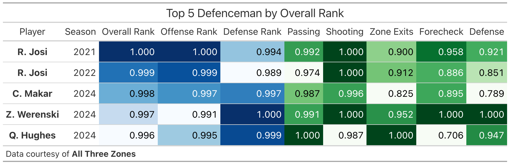
Top 5 seasons over the past 4 seasons by position

Player Projection Model
To project player impact (overall rank) in 2025-2026, I trained a Long Short-Term Memory (LSTM) model, a neural network architecture designed to predict the next item in a sequence.
The archetypal LSTM typically analyzes sequences to predict the next item. However, this approach is problematic for player projection as it inherently disregards the crucial role of age. For instance, younger players, still developing, are more likely to sustain improvement than older players. To account for this, I incorporated a separate age pathway that processes a player's age and integrates their stage within three hard-coded career periods: development (18-25), prime (26-30), and decline (30+).

.
.